Basic equations and techniques
过去几十年中,人们发展了多种数值方案来求解描述宇宙重子成分与无碰撞暗物质的耦合方程组。绝大多数重子(即气体)可被描述为理想流体,其演化由一组方程——即欧拉方程——所支配。积分上述方程的流体求解器可归为两大类,如Fig. 2所示:粒子方法(离散化质量,见[47]
及其参考文献)和网格方法(离散化计算域,见[48]
及其参考文献)。近年来又涌现出新的求解器:它们融合了两种方法的特征(见[49]
及其参考文献),将在后续章节中详细讨论。
A variety of numerical schemes has been developed in the past decades to solve the coupled system of equations describing the baryonic content of the Universe and the collisionless DM. The majority of the baryons (i.e. gas) can be described as an ideal fluid, whose evolution is ruled by a set of equations, namely, the Euler equations. The hydro solvers which integrate the aforementioned equations fall into two main categories, that are summarized in Fig. 2: particle methods, which discretize mass (see [47]
and references therein), and grid-based methods, which discretize the computational domain (see [48]
and references therein). Recently, additional solvers have been developed: they combine characteristics of both methods (see [49]
and references therein) and will be discussed in detail in the following sections.
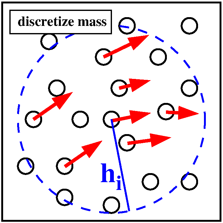 拉格朗日描述 | 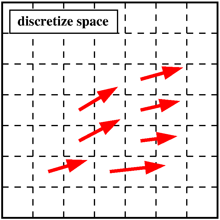 欧拉描述 |
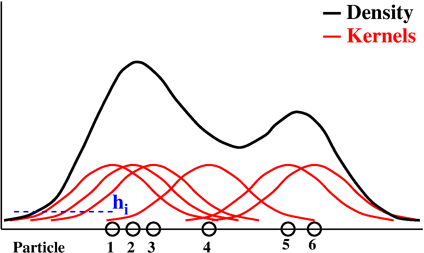 核密度估计 | 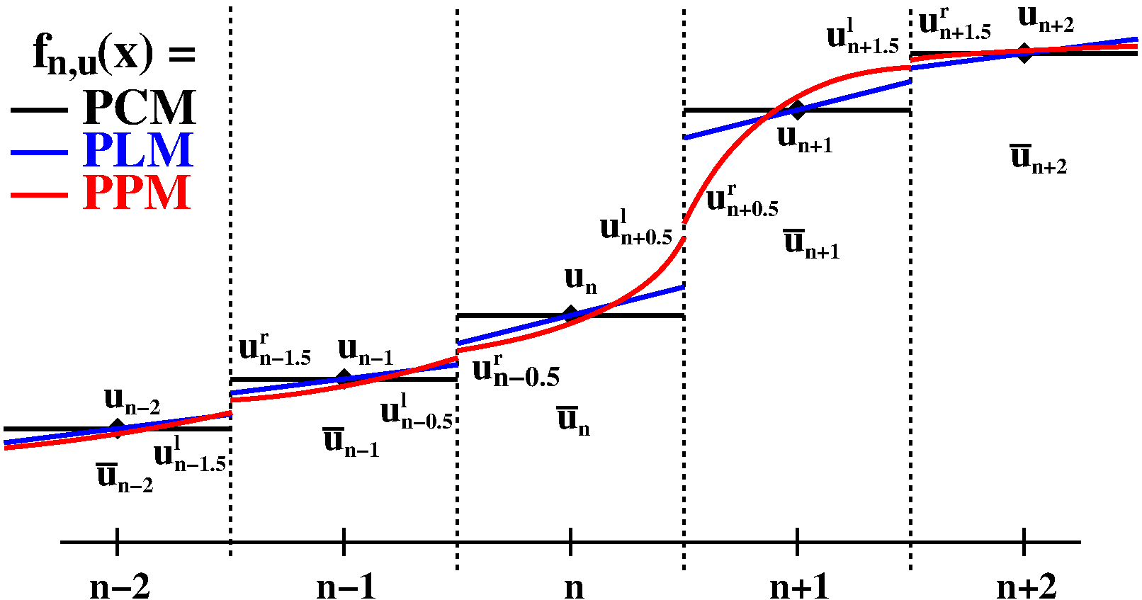 网格划分 |
所有求解器均需通过状态方程来封闭,该方程将气体压强 $P$ 与(单位质量)内能 $u$ 及密度 $\rho$ 联系起来。假设为理想单原子气体,则有 $P = (\gamma - 1) \rho u$,多方指数 $\gamma = 5/3$。
All of them have to be closed by an equation of state, relating the gas pressure P to the internal energy (per unit mass) u and the density ρ. Assuming an ideal, monoatomic gas, this will be P = (γ−1) ρ u with the polytropic index γ = 5/3.
将这些方程应用于宇宙学结构形成问题时,与在非膨胀背景下的纯流体动力学模拟相比,会浮现出几个新的特征。首先,通常被忽略的自引力(表现为 $\nabla \Phi$ 项)必须纳入考量(其贡献可按 $N$ 体章节中描述的方法求解)。
When applying these equations to the problem of cosmological structure formation, there are several features emerging in comparison to purely hydrodynamic simulations in a non-expanding background. First, the otherwise often neglected self-gravity, emerging as the ∇Φ term, has to be accounted for (its contribution can be solved following the methods described in N体章节).
其次,辐射损失——通过冷却函数 $\Lambda(u, \rho)$ 量化,其中 $n^2 \Lambda$($n^2 \Lambda / \rho$)表示单位体积(质量)的冷却率,$n$ 为气体数密度——对重子成分的演化起着关键作用(亦见 §3.11)。冷却对描述宇宙恒星形成历史尤为关键,如 §3.14 所述。
Second, radiative losses, quantified through the cooling function Λ(u,ρ), where n²Λ (n²Λ/ρ) represents the cooling rate per unit volume (mass), with n being the gas number density, play a key role in influencing the evolution of the baryonic component (see also Section 11). Cooling is especially key to describe the history of star formation of the Universe, as outlined in Section 14.
此外,方程必须适配宇宙学背景(即计入宇宙的膨胀历史)。在几乎所有情形中,这最后一步都是通过切换到所谓的共动坐标并变换时间变量来实现的。这一改变通常不改变前述方程的一般结构,只是方程中会出现额外的、依赖于宇宙学时间的因子(关于严格推导,建议读者参阅[50]
第5章)。
Additionally, the equations have to be adapted to the cosmological background (to take into account the expansion history of the Universe). In almost all cases, the latter step is achieved by switching to the so called comoving coordinates and through a transformation of the time variable. This change does not typically alter the general structure of the equations above, except for additional, cosmological, time dependent pre-factors which appear in the equations (we refer the reader to chapter 5 in [50]
for a rigorous derivation).
系列导航
← 上一篇:§3.2 流体动力学与数值方法
→ 下一篇:§3.4 欧拉网格方法
评论