Eulerian (grid) methods
网格方法在结构或非结构化网格上求解欧拉方程(参见Fig. 2),用以表示流体。其中,原始变量描述流体的热力学性质(如 $\rho$、${\vec v}$ 或 $P$),而守恒变量则定义守恒定律(如 $\rho$、$\rho{\vec v}$ 或 $\rho u$)。早期研究者尝试使用中心差分格式:流体仅以网格中心的数值表征,导数则通过有限差分表示求得(参见例如 [51]
)。这些方法采用人工黏性来处理激波(类似于§3.6中描述的平滑粒子流体动力学方法),否则在出现间断的区域会失效。此外,从构造上讲,它们仅具有一阶精度。
Grid-based methods solve the Euler equations (see Fig. 2) based on structured or unstructured grids, representing the fluid.
While primitive variables encode the thermodynamic properties of the fluid (e.g., $\rho$, ${\vec v}$, or $P$), conservative variables define the conservation laws (e.g., $\rho$, $\rho{\vec v}$, or $\rho u$).
Early attempts were made using a central difference scheme, where fluid is only represented by the centered cell values and derivatives are obtained by the finite-difference representation (see, for example, [51]
). These methods use artificial viscosity to handle schocks (similar to the smoothed particle hydrodynamics method described in §3.6), as they would otherwise break down in regimes where discontinuities appear. Also, by construction, they are only first-order accurate.
经典方法则采用重构格式,根据其阶数,利用数个相邻网格(即所谓的模板点)来重构任意流体力学变量($u_n$)的场,从而在网格界面($u_{\pm0.5}^{l/r}$)处逐步提高精度阶数。典型的格式包括分段常数方法(PCM)、分段线性方法(PLM;如 [52]
)和分段抛物线方法(PPM;[53]
),如Fig. 2右下部分所示。然后,利用重构函数的形状来计算某个物理量在网格单元上的总积分除以每个网格的体积(即网格平均值,${\bar u}_n$),而非在网格中心处做逐点近似(即中心变量,$u_n$)。
Classical approaches use instead reconstruction schemes which, depending on their order, take several neighboring cells (so-called stencils) into account to reconstruct the field of any hydrodynamical variable ($u_n$), with increasing order of accuracy at the interfaces of the cells ($u_{\pm0.5}^{l/r}$).
Typical schemes are the piecewise constant method (PCM), the piecewise linear method (PLM; e.g., [52]
), and the piecewise parabolic method (PPM; [53]
), as illustrated in the lower right part of Fig. 2. The shape of the reconstruction function is then used to calculate the total integral of a quantity over the grid cell, divided by the volume of each cell (e.g., cell average, ${\bar u}_n$), rather than pointwise approximations at the grid centers (e.g., central variables, $u_n$).
Modern, high-order schemes usually have stencils based on at least five grid points and implement essentially nonoscillatory (ENO; [54]
) or the so-called weighted essentially nonoscillatory (WENO; [55]
) schemes for reconstruction, which maintain high-order accuracy (see e.g., [56]
for a recent review).
重构后的物理量用于计算网格边界左侧和右侧的值。这些值随后用作初始条件来求解所谓的Riemann问题(见Fig. 3右图),其解给出穿过网格边界的各种物理量(如质量、能量等)的通量。此外,还需引入额外约束以抑制重构中的振荡(例如避免出现新的极值),即所谓的斜率限制器,用于估计重构所允许的最大斜率。一种方法是要求界面间的总变差不随时间增加。这些所谓的总变差递减格式(TVD;[57]
)如今提供了多种不同的斜率限制器,由不同作者提出。
The reconstructed quantities are used to calculate the left- and right-hand side values at the cell boundaries. These values are then exploited as initial conditions to solve the so-called Riemann problem (see right panel of Fig. 3), whose solution provides the fluxes of various quantities (e.g., mass, energy, etc.) across the cell borders. Additional constraints are included to avoid oscillations (e.g., the development of new extrema) in these reconstructions, such as the so-called slope limiters, which estimate the maximum slope allowed for the reconstruction. One way is to demand that the total variation among the interfaces does not increase with time. These so-called total variation diminishing schemes (TVD; [57]
) nowadays provide various different slope limiters, as suggested by different authors.
 初始状态 | 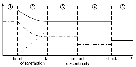 最终状态 |
如何求解一般Riemann问题——即初始分隔两种状态的间断的演化——可参见教科书(如 [58]
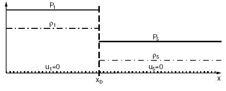
)。这里,我们仅以激波管为例做简要描述。这对应于一个初始时刻两侧都处于静止的系统。Fig. 3的左侧部分显示了初始(上图)和演化后(下图)的系统。后者可划分为五个区域。区域1和5的值与初始构型相同。区域2是一个稀疏波,由区域1和区域3的状态决定。求解此问题可借助一般的Rankine--Hugoniot条件,该条件描述了间断处的跳跃关系。它们列在右上部分,其中我们假设了一个随激波速度 $v_s$ 运动的坐标系。结合这些条件并定义初始密度比 $\lambda=\rho_1/\rho_5$,可得到关于压力比 $P=P_{3,4}/P_5$ 的非线性代数方程,如Fig. 3右下部分所示。一旦求解该方程得到 $P_{3,4}$,其余未知量便可从四个条件中逐步导出。
How to solve the general Riemann problem, i.e. the evolution of a discontinuity initially separating two states, can be found in textbooks (e.g., [58]
).
Here, we only want to give a brief description of the solution of a shock tube as an example.
This corresponds to a system where both sides are initially at rest. The left part of Fig. 3 shows in the initial (upper panel) and the evolved (lower panel) system. The latter can be divided into five regions. The values for regions 1 and 5 are identical to the initial configuration. Region 2 is a rarefaction wave which is determined by the states in regions 1 and 3.
The solution can be obtained by invoking the general Rankine--Hugoniot conditions, describing the jump conditions at a discontinuity. They are listed in the right upper part, where we have assumed a coordinate system which moves with the shock velocity $v_s$. By combining such conditions and defining the initial density ratio $\lambda=\rho_1/\rho_5$, it is possible to get the nonlinear, algebraic equation for the pressure ratio $P=P_{3,4}/P_5$, as displayed in the lower right part of Fig. 3. Once $P_{3,4}$ is known by solving this equation, the remaining unknowns can be inferred step by step from the four conditions.
在流体力学代码中精确求解Riemann问题可能代价高昂,并严重影响代码性能。因此,有多种近似方法可用于求解Riemann问题,包括所谓的ROE方法(如 [59]
)、HLL/HLLE方法(如参见 [60]
、[61]
、[62]
)以及HLLC(如参见 [63]
)。对所有方法的详细描述超出了本综述的范围,请读者参阅所引文献或教科书(如 [64]
)。
Solving the full Riemann problem in a hydrodynamics code can be expensive and it can severely affect the code performance. Therefore, there are various approximate methods to solve the Riemann problem, including the so-called ROE method (e.g., [59]
), the HLL/HLLE method (e.g., see [60]
,[61]
,[62]
), and HLLC (e.g., see [63]
). A description of all these methods is outside the scope of this review, so we refer the reader to the references given or to textbooks (e.g., [64]
).
宇宙学应用中采用了多种网格代码,包括基于TVD的代码(如 [65]
和 CosmoMHD [66]
)以及基于PLM的代码(如 ART [67]
、[68]
和 RAMSES [69]
)。基于PPM的代码包括 Zeus [70]
、ENZO [71]
、COSMOS [72]
和 FLASH [73]
。值得指出基于WENO的代码 [74]
。
A wide variety of grid codes are used for cosmological applications, including TVD-based codes (e.g., [65]
and CosmoMHD [66]
) and PLM-based codes (like ART [67]
,[68]
and RAMSES [69]
).
PPM-based codes include Zeus [70]
, ENZO [71]
, COSMOS [72]
, and FLASH [73]
.
It is worth mentioning the WENO-based code by [74]
.
系列导航 ← 上一篇:§3.3 基本方程与技术 → 下一篇:§3.5
评论