Lagrangian methods and Smoothed Particle Hydrodynamics
SPH的基本思想是用质量元(即粒子)而非像Euler方法那样用体积元来离散流体(参见Fig. 2)。显然,已坍缩天体中的平均粒子间距小于低密度区域。因此,该方案通过保持质量分辨率固定,实现了空间分辨率的自适应。关于SPH格式的全面综述及其严格推导,参见[47]
。
The basic idea of SPH is to discretize the fluid by mass elements (i.e. particles), rather than by volume elements as in Eulerian methods (see Fig. 2). It is evident that the mean interparticle distance in collapsed objects is smaller than in underdense regions. The scheme will thus be adaptive in spatial resolution by keeping the mass resolution fixed. For a comprehensive review with rigorous derivations of the SPH formalism, see [47]
.
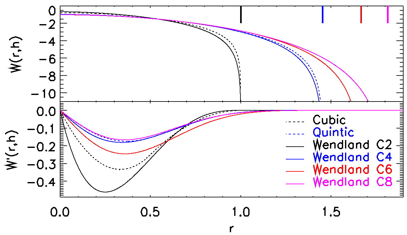
Fig. 5总结了SPH的主要特征。核函数光滑方法的一般定义,是为任意变量$X$构建连续流体量的第一步。其中,核函数仅依赖于距离的模,同时还要求是单调且可微的(参见Fig. 5上部)。在离散化形式中,我们将积分的体积元$d {\vec x} = d^3 x$替换为粒子的质量与密度之比$m_j/\rho_j$。虽然该方程对空间中的任意位置${\vec x}$都成立,但这里我们只关心原始粒子位置${\vec x}_i$处的流体表示,这些位置是后面唯一需要流体表示的地方。需要注意的是,对于具有紧支撑的核函数(即当$|{\vec x}|>h$时$W({\vec x},h)=0$),求和无需对所有粒子进行,而只需对半径为$h$的球体内的粒子(参见Fig. 2)——即所考虑粒子$i$周围的邻居粒子——进行求和。最初,最常用的核函数是$B_2$样条,但现代方法采用了全新的核函数族,如HOCT核函数[80]
或所谓的Wendland核函数[81]
,它们表现出更好的稳定性和更高的精度(参见Fig. 5右上图和[82]
的最新综述及其参考文献)。
Fig. 5 summarizes the main characteristics of SPH.
The general definition of a kernel smoothing method is the first step to build continuous fluid quantities for an arbitrary variable $X$. Here, the kernel depends on the distance modulus only, and is in addition required to be monotonic and differentiable (see upper part of Fig. 5). In the discretized version, we replace the volume element of the integration, $d {\vec x} = d^3 x$, with the ratio of the mass and density $m_j/\rho_j$ of the particles. Although this equation holds for any position ${\vec x}$ in space, we are only interested here in the fluid representation at the original particle positions ${\vec x}_i$, which are the only locations where we will need the fluid representation later on. It is important to note that for kernels with compact support (i.e., $W({\vec x},h)=0$ for $|{\vec x}|>h$), the summation does not have to be done over all the particles but only over the particles within the sphere of radius $h$ (see Fig. 2), namely, the neighbors around the particle $i$ under consideration. Originally, the most frequently used kernel is the $B_2$-Spline, but modern schemes invoke an entire new family of kernels like the HOCT kernels [80]
or the so-called Wendland kernels [81]
which show better stability and higher accuracy (see upper right panel of Fig. 5 and also recent review by [82]
and references therein).
导数可利用核函数的解析导数来计算。当使用成对对称公式时,守恒定律在数值上可得到更好的满足:这可通过在利用$\rho X$或$X/\rho$的导数时引入一些恒等式来实现(参见Fig. 5左中部)。为利用SPH方法的自适应特性,通常允许每个粒子$i$具有不同的光滑长度$h_i$,并通过在核函数内包含固定数量的邻居粒子或固定质量来确定。然而,上述独立光滑长度常常带来两方面的复杂性:首先,成对对称公式需要为每对粒子定义一个平均核函数,历史上已提出过各种构建平均值的方法。其二,核函数的导数——因光滑长度在空间上变化——伴随着修正项($\partial h_i/\partial \rho_i$),这些修正项最初总被忽略,因其无法直接计算。从熵表述出发,[83]
首次从拉格朗日形式导出了包含变化光滑长度的适当修正项的SPH公式,这些公式列在Fig. 5的右中部。注意,该形式同时也规定了粒子对平均核函数的构造方式。
Derivatives can be calculated using the analytically known derivatives of the kernel. Conservation laws are numerically better achieved when pairwise symmetric formulations are used: this can be obtained by exploiting some identities when using derivatives of $\rho X$ or $X/\rho$ (see left middle part of Fig. 5). To profit from the adaptive nature of the SPH method, the smoothing length $h_i$ is typically allowed to vary for each individual particle $i$ and is determined by encompassing either a fixed number of neighbours or a fixed mass within the kernel. However, two complications often stem from the abovementioned individual smoothing lengths: first, a pairwise symmetric formulation needs to define an averaged kernel for each particle pair, and historically various ways to build averages have been discussed. The other is that the derivatives of the kernel -- being the smoothing length spatial dependent -- come with correction terms ($\partial h_i/\partial \rho_i$), which originally have been always ignored because they can't be computed directly. Starting from an entropy formulation, [83]
derived for the first time an SPH formulation including the proper correction terms for the varying smoothing length from a Lagrangian formalism, which are listed in the middle right part of Fig. 5. Note that this formalism then also specifies the way in which the averaged kernel for a particle pair has to be constructed.
这还可进一步推广,如[84]
所示。在该工作中,从$x$加权的体积平均
$$
\bar{y} = y_i = \sum_j x_j W_{ij}(h_i),
$$
($x$加权的)体积元$\Delta\nu_i\equiv x_i/y_i$以及压强$P_i$、单位质量内能$u_i$和熵函数$A_i$之间的广义关系
$$
P_i = (\gamma-1)u_i\frac{m_i}{\Delta\nu_i} = A_i\left(\frac{m_i}{\Delta\nu_i}\right)^\gamma
$$
出发,得到了这一广义公式。由此导出广义SPH方程组
$$
m_i \frac{d {\vec v}_i}{d t} = - \sum_j x_i x_j \left(f_{ij}\frac{P_j}{y_j^2}{\vec \nabla}_i W_{ij}(h_i) + f_{ji}\frac{P_i}{y_i^2}{\vec \nabla}_i W_{ij}(h_j) \right)\!,
$$
和
$$
f_{ij} \equiv 1 - \frac{\tilde{x_i}}{x_j} \left(\frac{h_i}{3\tilde{y_i}} \frac{\partial y_i}{\partial h_i}\right) \left[1 + \frac{h_i}{3\tilde{y_i}}\frac{\partial \tilde{y_i}}{\partial h_i}\right]^{-1}.
$$
当取$x_i=\tilde{x_i}=m_i$时,有$y_i=\tilde{y_i}=\bar{\rho_i}$和$\Delta\nu_i=m_i/\rho_i$,并遵循熵$A_i$(即$P_i=A_i\bar{\rho_i}^\gamma$),这组方程将给出[83]
中提出的熵守恒SPH公式。当取$x_i=\tilde{x_i}=(\gamma-1)m_i u_i$时,有$y_i=\bar{P_i}$和$\Delta\nu_i=(\gamma-1)m_i u_i/P_i$,这将给出[85]
中提出的压强-能量SPH公式。由于此时压强是核函数加权的量,接触间断面便得到了正确处理。第三种可能性是取$x_i=m_iA_i^{1/\gamma}$,它将导出压强-熵公式。更多细节见[84]
。
This can be further generalized, as shown in [84]
. There, such a generalized formulation was obtained starting from an x-weighted volume average
$$
\bar{y} = y_i = \sum_j x_j W_{ij}(h_i),
$$
the (x-weighted) volume element $\Delta\nu_i\equiv x_i/y_i$ and the generalized relation
$$
P_i = (\gamma-1)u_i\frac{m_i}{\Delta\nu_i} = A_i\left(\frac{m_i}{\Delta\nu_i}\right)^\gamma
$$
between the pressure $P_i$, the internal energy per unit mass $u_i$ and the entropic function $A_i$. This leads to the set of generalized SPH equations
$$
m_i \frac{d {\vec v}_i}{d t} = - \sum_j x_i x_j \left(f_{ij}\frac{P_j}{y_j^2}{\vec \nabla}_i W_{ij}(h_i) + f_{ji}\frac{P_i}{y_i^2}{\vec \nabla}_i W_{ij}(h_j) \right)\!,
$$
and
$$
f_{ij} \equiv 1 - \frac{\tilde{x_i}}{x_j} \left(\frac{h_i}{3\tilde{y_i}} \frac{\partial y_i}{\partial h_i}\right) \left[1 + \frac{h_i}{3\tilde{y_i}}\frac{\partial \tilde{y_i}}{\partial h_i}\right]^{-1}.
$$
For the choice of $x_i=\tilde{x_i}=m_i$, which implies $y_i=\tilde{y_i}=\bar{\rho_i}$ and $\Delta\nu_i=m_i/\rho_i$, and following the entropy $A_i$ (e.g., $P_i=A_i\bar{\rho_i}^\gamma$), this set of equations will result in the entropy-conserving formulation of SPH as presented in [83]
. For the choice of $x_i=\tilde{x_i}=(\gamma-1)m_i u_i$, implying $y_i=\bar{P_i}$ and $\Delta\nu_i=(\gamma-1)m_i u_i/P_i$, this results in a pressure--energy formulation of SPH, as presented in [85]
. As now pressure is a kernel weighted quantity, contact discontinuities are properly treated. A third possibility is to choose $x_i=m_iA_i^{1/\gamma}$ which leads to a pressure--entropy formulation. For more
details, see [84]
.
然而,SPH方法在低密度区域的表现不如高密度区域。由于引入了可观的人工黏性,它在激波区域的分辨率也会下降。在其经典实现中,离散化误差会在密度梯度陡峭的区域——特别是在接触间断面附近——对粒子引入虚假压力。这导致了一个尺度为SPH光滑核函数半径的边界间隙,该间隙内的相互作用受到严重阻尼。标准实现通常不包含显式的混合项来补偿这种效应。因此,经典实现无法分辨和处理多相流体相互作用中的动力学不稳定性,如Kelvin-Helmholtz不稳定性或Rayleigh-Taylor不稳定性。这两个缺点均可通过本节末尾描述的现代实现来克服。此外,在宇宙学背景下,SPH方法的自适应特性、其与引力的简单耦合方式以及可使用独立时间步长的能力,常常弥补了这些不足,从而使SPH仍为数值流体宇宙学中最常用的方法之一。
The SPH method, however, is not performing as well in low-density regions as in the higher density ones. It also suffers from degraded resolution in shocked regions due to the introduction of a sizeable artificial viscosity. In its classical implementation, discretization errors introduce spurious pressure forces on particles in regions with steep density gradients in particular near contact discontinuities. This results in a boundary gap of the size of an SPH smoothing kernel radius over which interactions are severely damped. The standard implementation typically does not involve an explicit mixing term, which can compensate this effect. Therefore, the classical implementation does not resolve and treat dynamical instabilities in the interaction of multi-phase fluids, such as Kelvin--Helmholtz or Rayleigh--Taylor instabilities. Both these shortcomings can be overcome by a modern implementation as described at the end of this section. In addition, in the cosmological context, the adaptive nature of the SPH method, its simple way to couple to gravity and the possibility to have individual time steps often compensate for such shortcomings, thus making SPH still one of the most commonly used methods in numerical hydrodynamical cosmology.
如前所述,还需添加所谓的人工黏性$\Pi_{ij}$,使得熵守恒SPH公式的最终方程为
$$
\frac{d {\vec v}_i}{d t} = - \sum_j m_j \left(f_j\frac{P_j}{\rho_j^2}{\vec \nabla}_i W_{ij}(h_j)+f_i\frac{P_i}{\rho_i^2}{\vec \nabla}_i W_{ij}(h_i) +
\Pi_{ij} {\vec \nabla}_i {\bar W}_{ij} \right),
$$
以及
$$
\frac{d A_i}{d t} = \frac{1}{2} \frac{\gamma-1}{\rho_i^{\gamma-1}} \sum_j m_j \Pi_{ij}
\left({\vec v}_j - {\vec v}_i\right){\vec \nabla}_i {\bar W}_{ij}.
$$
这一描述人工黏性的项通常是捕捉激波所必需的,其构造方式与其他流体动力学格式类似。流行的公式有Monaghan和Gingold[86]
以及Balsara[87]
提出的形式,这些公式包含体黏性项和von Neumann-Richtmeyer黏性项,并辅以限制器以减少低粒子数下剪切流中的角动量输运[88]
。现代方法采用[89]
提出的人工黏性形式,它基于可压缩气体动力学Riemann解的类比。为减少至少无激波流动区域中的人工黏性,一种可行途径是遵循Morris和Monaghan[90]
提出的思想:每个粒子携带自己的人工黏性,该黏性在激波区域之外会逐渐衰减。关于这种实现对ICM的影响的详细研究可参见[91]
。在高阶人工耗散项的实现方面还有各种进一步的改进[92]
,[93]
。现代SPH公式还利用了速度梯度的高阶计算方案,参见Fig. 5下部以及[94]
,[95]
中的相关讨论。通过采用[92]
并辅以这种速度梯度的高阶计算方案,可更好地抑制人工黏性,如[96]
所示。
This term describing an artificial viscosity is usually needed to capture shocks and its construction is similar to other hydrodynamical schemes. Popular formulations are those proposed by Monaghan and Gingold [86]
and Balsara [87]
, which includes a bulk viscosity and a von Neumann--Richtmeyer viscosity term, supplemented by a limiter reducing angular momentum transport in the presence of shear flows at low particle numbers [88]
. Modern schemes implement a form of the artificial viscosity as proposed by [89]
, based on an analogy with Riemann solutions of compressible gas dynamics. To reduce this artificial viscosity, at least in those parts of the flows where there are no shocks, a posibility is to follow the idea proposed by Morris and Monaghan [90]
: every particle carries its own artificial viscosity, which eventually decays outside the regions which undergo shocks. A detailed study of the implications on the ICM of such an implementation can be found in [91]
. There are various further improvements on the implementation a higher order artificial dissipation term [92]
,[93]
. Modern SPH formulations also make use of higher order calculation schemes for velocity gradients, see lower part of Fig. 5 as well as related discussion in [94]
,[95]
. Even better suppression of the artificial viscosity can be reached by following [92]
in combination with such higher order calculation schemes for velocity gradients, as shown in [96]
.
过去十年中,研究者付出了相当大的努力来结合Lagrange方法和Euler方法的优势。一方面,将Godunov方法引入SPH形式取得了显著进展,参见[97]
,[98]
,[99]
,[100]
,这些工作最近促成了所谓的无网格方法的诞生。另一方面,在将Euler方法推广到移动网格方法方面也付出了巨大努力。这两种新方法将在接下来的两个小节中简要介绍。
Considerable effort has been made in the last decade to combine the advantages of Langrangian and Eulerian methods. On one hand, significant progress has been achieved in involving Godunov methods into the SPH formalism, see [97]
,[98]
,[99]
,[100]
, which recently led to the so called meshless methods. On the other hand, large effort has been made to extend Eulerian methods to moving mesh methods. Both these new methods are briefely described in the next two sub-sections.
评论