Moving mesh methods
研究者投入了大量精力,将§3.4中描述的Euler方法重新表述为Lagrange网格方法。移动网格流体动力学在宇宙学中应用的更多细节,可参见[101]
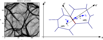
的开创性工作及其参考文献。这种早期方法从规则网格出发,然后通过跟随流体流动使网格变形。Euler方程通过计算网格边界上的通量来演化。宇宙学模拟中得到的网格示例见Fig. 6左图。该技术在实际应用中的一个缺点(或挑战)是单个网格单元可能严重变形和拉伸。现代方案通过基于Voronoi或Delaunay镶嵌构建非结构网格,规避了这一问题(参见[102]
及其参考文献)。基于网格生成点$\vec{r}_i$和$\vec{r}_j$的网格单元相关几何结构如Fig. 6右图所示。然后必须在界面的质心处计算通量(注意,该质心不一定位于两个网格生成点之间的直线上,如虚线所示)
$$
\mathbf{Q}_i^{(n+1)} = \mathbf{Q}_i^{(n)} - \Delta t \sum_j A_{ij}\hat{\mathbf{F}}_{ij}^{(n+1/2)}.
$$
该界面的运动$\vec{w}$由速度$\vec{w}_i$和$\vec{w}_j$唯一定义,并且必须在旋转坐标系($x',y'$)中使用Riemann求解器计算通量。该技术的详细描述及其在测试问题中的表现,可参见[102]
。
Substantial effort has gone into reformulating Eulerian methods as described in §3.4 into Lagrangian mesh approaches. More details on the idea of hydrodynamics on moving mesh for cosmological application can be found in the pioneering work by [101]
and references therein. This early approach started from a regular mesh which then, by following the flow of the fluid, was deformed. The Euler equations were evolved by calculating the fluxes across the cell borders. An example of the resulting mesh for a cosmological simulation can be seen in the left part of Fig. 6. One disadvantage (or challenge) of this technique in practical applications is that individual cells can be extensively deformed and stretched. Modern schemes circumvent this problem by constructing an unstructured mesh based on a Voronoi or Delaunay tessellation (see [102]
and references therein). The relevant geometry of the cells, based on the mesh generating points $\vec{r}_i$ and $\vec{r}_j$ is illustrated in the right part of Fig. 6. The fluxes then have to be calculated at the centroid of the interface (note that this is not necessarily on the straight line between the two mesh generating points, as indicated by the dotted line)
$$
\mathbf{Q}_i^{(n+1)} = \mathbf{Q}_i^{(n)} - \Delta t \sum_j A_{ij}\hat{\mathbf{F}}_{ij}^{(n+1/2)}.
$$
The motion $\vec{w}$ of this interface is uniquely defined by the velocities $\vec{w}_i$ and $\vec{w}_j$, and the fluxes have to be calculated with the Riemann solver in the rotated frame ($x',y'$). A detailed description of this technique along with its performance in test problems can be found in [102]
.
评论