Meshless methods
最近,一类新的拉格朗日方法——即所谓的无网格公式——在天体物理领域得到了发展。更多细节见[102]
、[104]
、[105]
,这些工作继承了[106]
、[107]
、[108]
更早的开创性研究。简而言之,推导从积分形式
$$
\int[u(\vec{x},t)\dot\phi(\vec{x},t) + \vec{F}(u,\vec{x},t)\cdot\nabla\phi(\vec{x},t) + S(\vec{x},t)\phi(\vec{x},t)]\,d\vec{x}\,dt = 0
$$
出发,它是标量守恒律
$$
\frac{\partial u}{\partial t} + \nabla\cdot(\vec{F} + \vec{a}u) = S
$$
的积分形式。其中,$u(\vec{x},t)$是一个标量场,$S(\vec{x}, t)$是其源项,$\vec{F}(u,\vec{x},t)$是在以速度$\vec{a}(\vec{x}, t)$运动的参考系中的通量,而$\phi(\vec{x},t)$是空间和时间上的任意可微函数,由此定义了随体导数$\dot\phi(\vec{x}, t) = \partial\phi(\vec{x}, t)/\partial t + \vec{a}(x,t)\cdot\nabla\phi(\vec{x}, t)$。
A new class of Lagrangian methods, the so-called meshless formulations, have been recently developed for astrophysical problems. More details can be found in [102]
,[104]
,[105]
, which follow earlier, pioneering work by [106]
,[107]
,[108]
. In short, the derivation starts from the integral form
$$
\int[u(\vec{x},t)\dot\phi(\vec{x},t) + \vec{F}(u,\vec{x},t)\cdot\nabla\phi(\vec{x},t) + S(\vec{x},t)\phi(\vec{x},t)]\,d\vec{x}\,dt = 0
$$
of a scalar conservation law
$$
\frac{\partial u}{\partial t} + \nabla\cdot(\vec{F} + \vec{a}u) = S \,.
$$
Here, $u(\vec{x},t)$ is a scalar field, $S(\vec{x}, t)$ is its source, $\vec{F}(u,\vec{x},t)$ is its flux in a frame moving with velocity $\vec{a}(\vec{x}, t)$, and $\phi(\vec{x},t)$ is an arbitrary differentiable function in space and time leading to the advective derivative $\dot\phi(\vec{x}, t) = \partial\phi(\vec{x}, t)/\partial t + \vec{a}(x,t)\cdot\nabla\phi(\vec{x}, t)$.
采用与SPH类似的做法,以一组粒子$i$进行离散(光滑长度为$h(\vec{x})$,核函数为$W(\vec{x},h)$),则粒子划分可写为
$$
\psi_i(\vec{x}) = w(\vec{x})W(\vec{x}-\vec{x}_i,h(\vec{x})),
$$
其中粒子的数密度为$w(\vec{x})^{-1} = \sum_j W(\vec{x}-\vec{x}_j,h(\vec{x}))$。任意函数$f(\vec{x})$的离散化可写为
$$
\int f(\vec{x})\,d\vec{x} \approx \sum_i f_i \int \psi_i(\vec{x})\,d\vec{x} \equiv \sum_i f_i
V_i,
$$
其中$V_i = \int \psi_i(\vec{x})\,d\vec{x}$是粒子$i$的有效体积。因此,积分方程(3.28)的离散形式可写为
$$
\sum_i \int [ V_i u_i \dot\phi_i + V_i F^\alpha_i (D^\alpha\varphi)_i + V_i S_i \phi_i ] = 0 \, .
$$
虽然原则上可采用$(D^\alpha\phi)_i$的SPH估计,但更方便的做法是采用[107]
建议的更精确的无网格梯度估计。结合第一项的分部积分,由此(如[102]
所示)可将$\phi(\vec{x}, t)$分离出来并得到:
$$
\frac{d}{dt}(V_i u_i) + \sum_j\left[V_i F_i^\alpha\psi_j^\alpha(\vec{x}_i) - V_j F_j^\alpha\psi_i^\alpha(\vec{x}_j)\right] = V_i S_i \, .
$$
该方程(及其对一般矢量场$\vec{u}$的推广)与移动网格方法的有限体积方程非常相似[Fn: 但注意,方程[eq:flux]是积分形式。],但在某种程度上也与SPH方程类似。其区别在于,不同粒子之间的相互作用由源项和通量项描述,而它们可通过求解粒子$i$和$j$之间的近似Riemann问题得到。进一步观察还可发现,实际只需粒子间连线方向上的投影,例如在中点处求解Riemann问题\footnote{更精确的做法是在核长度$h_i$和$h_j$的等分点处求积,参见[104]
中的讨论及其中的参考文献。}。这也意味着需要将原始变量外推到中点(例如使用线性外推),且通常还需施加通量限制器(参见[102]
、[104]
、[105]
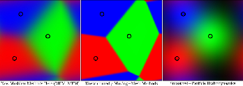
中的讨论)。Fig. 7展示了无网格方法、非结构(移动)网格和经典核加权形式(SPH)在体积划分上的差异。
Using a discretization through a set of particles $i$ with a smoothing length $h(\vec{x})$ and a kernel function $W(\vec{x},h)$, akin to what is done in SPH, the partitioning of the particles can be written as
$$
\psi_i(\vec{x}) = w(\vec{x})W(\vec{x}-\vec{x}_i,h(\vec{x})),
$$
where the number density of particles is $w(\vec{x})^{-1} = \sum_j W(\vec{x}-\vec{x}_j,h(\vec{x}))$. The discretization of an arbitrary function $f(\vec{x})$ can be written as
$$
\int f(\vec{x})\,d\vec{x} \approx \sum_i f_i \int \psi_i(\vec{x})\,d\vec{x} \equiv \sum_i f_i
V_i,
$$
where $V_i = \int \psi_i(\vec{x})\,d\vec{x}$ is the effective volume of a particle $i$. Therefore, the discrete form of the integral equation (3.28) can be written as
$$
\sum_i \int [ V_i u_i \dot\phi_i + V_i F^\alpha_i (D^\alpha\varphi)_i + V_i S_i \phi_i ] = 0 \, .
$$
Although in principle an SPH estimate for $(D^\alpha\phi)_i$ could be used, it is convenient to use a more accurate meshless gradient estimate, as suggested by [107]
. This, along with the integration of the first term by parts, makes it possible (as shown in [102]
) to split $\phi(\vec{x}, t)$ and to obtain:
$$
\frac{d}{dt}(V_i u_i) + \sum_j\left[V_i F_i^\alpha\psi_j^\alpha(\vec{x}_i) - V_j F_j^\alpha\psi_i^\alpha(\vec{x}_j)\right] = V_i S_i \, .
$$
This equation (and its extension to a general vector field $\vec{u}$) is very similar to the finite volume equation for the moving mesh method [Fn: Note that, however, Eq. [eq:flux] is in the integral form.] but also somewhat similar to the SPH equations, except that the interactions between different particles is described in the source and flux terms, which can be obtained as the solution of an approximate Riemann problem between particles $i$ and $j$. A closer inspection also reveals that only the projection on the direction between the particles is needed, e.g., the solution of the Riemann problem at the midpoint\footnote{More accurate would be the quadrature point at an equal fraction of the kernel length $h_i$ and $h_j$, see discussion in [104]
and references therein.}. This also means that the primitive variables have to be extrapolated to the midpoint, e.g., using linear extrapolation, and generally a flux limiter has to be applied (see discussion in [102]
,[104]
,[105]
). Fig. 7 illustrates the differences in partitioning the volumes between mesh-less methods, unstructured (moving) grid and classical kernel weighted formalism (SPH).
评论