Supermassive black holes in cosmological simulations
观测表明,几乎每个星系在其最内层区域都寄宿着一个超大质量($10^8\text{--}10^{10}\ M_{\odot}$)黑洞(SMBH)(例如,[231]
,[232]
,[233]
,[234]
,[235]
,[236]
,[237]
,[238]
,[239]
)。其中一部分黑洞表现出持续的活动性,称为活动星系核(AGN)。过去和当前活动的证据可见于椭圆星系、星系群和星系团的X射线图像,其中AGN的印记通常表现为凹陷和涟漪。在众多例子中,一个众所周知的代表是MS 0735+7421星系团的复合(X射线、射电和光学)图像(例如[240]
):巨大的X射线空洞充满射电辐射,并被Chandra图像中清晰可见的椭圆形茧状激波包围。
Observations suggest that almost every galaxy hosts a supermassive ($10^8\text{--}10^{10}\ M_{\odot}$) black hole (SMBH) in its innermost regions (e.g., [231]
,[232]
,[233]
,[234]
,[235]
,[236]
,[237]
,[238]
,[239]
). A fraction of these BHs exhibits ongoing activity and is called AGN (active galactic nuclei). Evidence of past and ongoing activity is observed for instance in the X-ray images of elliptical galaxies and galaxy groups and clusters, where AGN imprints often appear as depressions and ripples. Among many, a well-known example is represented by the composite (X-ray, radio, and visual) image of the MS 0735+7421 galaxy cluster (e.g. [240]
): giant X-ray cavities are filled with radio emission, and surrounded by a cocoon shock clearly visible in the Chandra image as an elliptical edge.
在讨论AGN反馈(见§3.16)之前,我们先回顾宇宙学模拟中黑洞的主要特征,重点关注黑洞种子植入与重定位、黑洞-黑洞并合以及AGN供料。
Before discussing AGN feedback (see §3.16), we are now recalling the main features of BHs in cosmological simulations, focusing on BH seeding and repositioning, BH-BH mergers, and AGN feeding.
大多数包含黑洞及相关AGN反馈的星系和星系团形成宇宙学模拟,都基于[241]
,[242]
的开创性黑洞模型,或秉承其思路。因此,该模型为讨论宇宙学模拟中黑洞处理的几个关键方面提供了基础,且凸显了最近的改进。
The majority of cosmological simulations of galaxy and galaxy cluster formation that also include BHs and the associated AGN feedback are based on the seminal BH model by [241]
,[242]
, or follow its spirit. Therefore, this model offers the base to discuss a few key aspects of the treatment of BHs in cosmological simulations, and to highlight recent improvements.
在宇宙学模拟中,通常将黑洞描述为汇粒子:这些是无碰撞粒子,可以吸收邻近元素(最初用于去除致密区域周围粒子,例如[243]
),且具有可直接与观测量关联的基本性质,如吸积率。
In cosmological simulations, BHs are usually described as sink particles: these are collisionless particles that can absorb neighbour elements (originally implemented to allow the removal of surrounding particles in dense regions, e.g. [243]
) and that have fundamental properties like the accretion rate which can be linked directly to observables.
在宇宙学模拟中,黑洞粒子于相对高红移处被植入大质量晕中,随后它们得以增长并增加其初始或{种子}质量。前述常引用的质量$M_{\bullet}$是黑洞的理论质量,在亚分辨率层次上建模,与之相对的是其动力学质量,即黑洞粒子的实际引力质量。由于我们对第一批超大质量黑洞的形成仍缺乏坚实理解(可能的形成途径见例如[244]
,[245]
,[246]
,[247]
,[248]
),且任何种子形成情景的物理过程都远超出当前分辨率所能企及,黑洞首先按种子植入方案插入(另见[249]
)。
BH particles are introduced in massive haloes at relatively high-redshift in cosmological simulations, and they are then allowed to grow and increase their initial or {seed} mass.
The aforementioned, commonly quoted mass $M_{\bullet}$ is the theoretical mass of the BH, modelled at the sub-resolution level, as opposite to its dynamical mass, i.e. the actual gravitational mass of the BH particle.
As we are still lacking a solid understanding of the formation of first SMBHs (see e.g., [244]
,[245]
,[246]
,[247]
,[248]
for possible pathways) and the resolution needed to take the physics of any seed formation scenario into account, BHs are first inserted according to seeding prescriptions (see also [249]
).
种子植入方案通常假设新的黑洞(质量约为$\sim 10^4\text{--}10^6\ M_{\odot}$ 的大质量种子)被植入满足某些条件且尚未包含黑洞的晕中。新黑洞的植入条件包括:$(i)$ 晕质量——通常通过FOF(Friend-Of-Friend,[250]
)算法估计——大于某个阈值(例如,[40]
,[41]
,[139]
,[6]
);$(ii)$ 恒星质量超过给定值(例如,[44]
);$(iii)$ 恒星质量以及气体与恒星质量之比大于给定阈值;$(iv)$ 基于气体性质,即气体密度、速度弥散和(或)金属丰度(例如,[251]
,[252]
,[253]
,[142]
)。植入时的黑洞质量可以是恒定的(例如,[40]
,[41]
,[139]
,[6]
,[44]
),也可以根据例如$M_{BH}$/$\sigma$或$M_{BH}$/$M_{\ast}$标度关系进行缩放(例如,[138]
)。进一步的细节涉及FOF算法所作用的粒子类型,例如可仅作用于暗物质粒子(例如,[254]
)或仅作用于恒星粒子(例如,[138]
)。此外,黑洞可植入在晕中最致密气体粒子的位置(例如,[254]
)、具有最大束缚能的恒星粒子的位置(例如,[138]
),或最接近结构质心的恒星粒子的位置(例如,[44]
)。
Seeding prescriptions usually assume that new BHs (massive seeds of $\sim 10^4\text{--}10^6\ M_{\odot}$) are introduced in haloes which meet some criteria and do not have already BHs.
New BHs are seeded if: $(i)$ the halo mass -- commonly estimated by means of a FOF (Friend-Of-Friend, [250]
) algorithm -- is larger than a threshold (e.g., [40]
,[41]
,[139]
,[6]
); $(ii)$ the stellar mass exceeds a given value (e.g., [44]
); $(iii)$ the stellar mass and gas to stellar mass fraction are larger than given thresholds; $(iv)$ based on gas properties, i.e. gas density, velocity dispersion and/or metallicity (e.g., [251]
,[252]
,[253]
,[142]
).
BH mass at seeding can be either constant (e.g., [40]
,[41]
,[139]
,[6]
,[44]
) or scaled according to e.g., the $M_{BH}$/$\sigma$ or $M_{BH}$/$M_{\ast}$ scaling relations (e.g., [138]
).
Additional details involve the type of particles on which the FOF algorithm is performed, whcih can be for instance DM particles only (e.g., [254]
) or stellar particles only (e.g., [138]
).
Besides, BH can be seeded at the position of the densest gas particle in the halo (e.g., [254]
), of the star particle with the largest binding energy (e.g., [138]
), or of the star particle closest to the centre of mass of the structure (e.g., [44]
).
在宇宙学模拟中,每个黑洞作为独立粒子经历特定的演化,这与N体模拟中通过粒子对无碰撞流体的粗粒化表示不同。因此,黑洞的动力学无法精确捕捉,数值伪迹会影响黑洞的运动(参见例如[255]
)。黑洞的虚假位移(通常源于高密度环境中的粒子间散射和数值加热)会带来严重后果,例如人为出现的游荡黑洞、对黑洞-黑洞并合的不正确描述、黑洞在偏离其星系宿主中心的位置产生反馈。为避免这些伪迹,黑洞动力学通常通过不同方法加以控制:通过钉扎进行重定位,如钉扎在最小势能处(例如,[40]
,[41]
,[139]
,[44]
)、增强动力学质量(例如,[144]
)、增强动力学质量与动力学摩擦(例如,[138]
,[145]
)。我们建议读者参考[254]
,[256]
,[35]
,[257]
,[143]
,[258]
,[249]
,[259]
,[260]
了解细节与近期改进。
In cosmological simulations, each BH undergoes a specific evolution as an individual particle, at variance with the coarse-grained representation of collisionless fluids through particles in N-body simulations. As a result, the dynamics of BHs fails to be accurately captured and numerical artefacts can affect BH motion (see e.g., [255]
). Spurious displacements of BHs, which often occur due to scattering between particles in high-density environments and numerical heating, have dramatic consequences, such as e.g., artificial presence of wandering BHs, incorrect description of BH-BH mergers, BHs producing feedback off-centre with respect to their galaxy hosts.
To avoid these artefacts, BH dynamics is commonly controlled through different approaches: re-positioning via pinning on e.g. minimum potential (e.g., [40]
,[41]
,[139]
,[44]
), boosted dynamical mass (e.g., [144]
), boosted dynamical mass and dynamical friction (e.g., [138]
,[145]
). We refer the reader to [254]
,[256]
,[35]
,[257]
,[143]
,[258]
,[249]
,[259]
,[260]
for details and recent improvements.
黑洞通过气体吸积以及与其他黑洞并合而增长。就后一种渠道而言,当黑洞的宿主星系及其晕并合形成单一结构时,黑洞预计会发生并合。宇宙学模拟中通常采用的方法[242]
,[241]
假设,如果两个黑洞粒子之间的距离接近模拟的空间分辨率(或其小的倍数),它们会快速并合。引力软化设定的力分辨率决定了能够正确追踪引力相互作用的最小尺度。还实现了涉及并合黑洞相对速度等的额外条件[254]
。两个黑洞最终并合成单个黑洞粒子,质量相加。
BHs grow because of gas accretion and mergers with other BHs.
As for the latter channel, BHs are expected to merge when their host galaxies and their haloes merge to form a single structure.
The commonly pursued approach [242]
,[241]
in cosmological simulations assumes that two BH particles merge quickly if their distance approaches the spatial resolution of the simulation (or a small multiple of it). The force resolution set by the gravitational softening determines indeed the minimum scale above which gravitational interactions can be properly followed. Additional conditions involving e.g. the merging BH relative speed have been implemented [254]
.
The two BHs are eventually merged into a single BH particle, with their masses combined.
对于AGN供料,质量为$M_{\bullet}$的黑洞的气体吸积率按Bondi公式[261]
,[262]
,[263]
计算,并乘以所谓的增强因子$\alpha$:
$$
\dot{M}_{B} = \frac{4 \pi \, \alpha \, G^2\, M_{\bullet}^2 \, \langle \rho \rangle}{(\langle
c_s\rangle^2 +\langle v\rangle ^2)^{3/2}} \,\, .
$$
As for AGN feeding, gas accretion onto a BH of mass $M_{\bullet}$ is calculated according to the Bondi formula [261]
,[262]
,[263]
, multiplied by a so-called boost factor $\alpha$:
$$
\dot{M}_{B} = \frac{4 \pi \, \alpha \, G^2\, M_{\bullet}^2 \, \langle \rho \rangle}{(\langle
c_s\rangle^2 +\langle v\rangle ^2)^{3/2}} \,\, .
$$
这里,$G$是引力常数,$\langle\rho\rangle$、$\langle v\rangle$和$\langle c_s\rangle$是流体动力学模拟可分辨尺度上的平均值:例如,在SPH情况下,它们通过核加权估计计算得到。黑洞吸积率$\dot{M}_{B}$通常受限于Eddington吸积率$\dot{M}_{Edd}$[Fn: $\dot{M}_{Edd}=(4\pi\:G\;m_p\; M_{\bullet})/(\sigma_T\;c\;\epsilon_r)$,其中$m_p$为质子质量,$\sigma_T$为Thompson散射截面,$c$为光速,$\epsilon_r$为辐射效率,通常取$\approx0.1$。](但超Eddington极限的$\dot{M}_{\bullet}$的例子见[264]
,[44]
)。
$$
Here, $G$ is the gravitational constant, $\langle\rho\rangle$, $\langle v\rangle$, and $\langle c_s\rangle$ are mean values at the scale resolved by the hydrodynamical simulation: for example, they are computed using kernel weighted estimates in the case of SPH.
The BH accretion rate $\dot{M}_{B}$ is commonly capped to the Eddington acccretion rate $\dot{M}_{Edd}$ [Fn: $\dot{M}_{Edd}=(4\pi\:G\;m_p\; M_{\bullet})/(\sigma_T\;c\;\epsilon_r)$, with $m_p$ the proton mass, $\sigma_T$ the Thompson cross section, $c$ the speed of light and
$\epsilon_r$ the radiative efficiency, typically assumed to be $\approx0.1$.] (but see [264]
,[44]
for examples of $\dot{M}_{\bullet}$ which breaches the Eddington limit).
增强因子$\alpha$最初引入[241]
是为了补偿模拟中有限的分辨率,这导致黑洞附近密度偏低、温度偏高(从而低估$\dot{M}_{B}$)。典型值为$\alpha =100$。多项研究通过采用依赖于分辨率[265]
,[266]
、密度[267]
或压力[268]
的增强因子来改进黑洞模型。其他模拟则通过考虑吸积气体的角动量来限制黑洞吸积率[269]
,[270]
。亚kpc尺度上的黑洞吸积高分辨率模拟[271]
发现,当包含冷却和湍流时,约100的增强因子是合适的,而纯绝热吸积则表明增强因子应小一个数量级。因此,更先进的模型区分热气与冷气吸积,并对两个组分使用不同的增强因子[272]
,甚至可以摆脱人为调节因子(例如,[139]
,[270]
)。
The boost factor $\alpha$ has been originally introduced [241]
to account for the limited resolution in simulations, which leads to smaller densities and larger temperatures near the BH (and thus to an underestimate of $\dot{M}_{B}$). A typical value is $\alpha =100$.
Several studies adapt the BH model by using a boost factor which depends on resolution [265]
,[266]
, density [267]
, or pressure [268]
. Other simulations instead limit the BH accretion rate by taking into account the angular momentum of accreting gas [269]
,[270]
.
High-resolution simulations of BH accretion on sub-kpc scales [271]
found that a boost factor of order of 100 is suitable when including cooling and turbulence, while pure adiabatic accretion suggests boost factors smaller by an order of magnitude. Hence, advanced models distinguish between hot and cold gas accretion and use different boost factors for the two components [272]
, or can even get rid of fudge factors (e.g., [139]
,[270]
).
利用黑洞吸积率$\dot{M}_{\bullet}$,可为模拟中的每个黑洞赋以热光度$L_{\mathrm bol}$。一个常见的假设是遵循[273]
,根据Eddington比$f_{Edd} = \dot{M}_{\bullet}/ \dot{M}_{Edd}$(即黑洞吸积率与Eddington吸积率之比)区分高吸积态和低吸积态,并计算:
$$
L_{\mathrm bol} =
\left\{
\begin{array}{ll}
10 \, ( \epsilon_r \; c)^2 \, \dot{M}_{\bullet} & f_{\mathrm Edd}>0.1 \\
(10 \, \epsilon_r\; c)^2 \, f_{\mathrm Edd}\; \dot{M}_{\bullet}\;\; & f_{\mathrm Edd}\leq0.1
\end{array} \right.
$$
(见[274]
,[275]
)。与原始模型[242]
,[241]
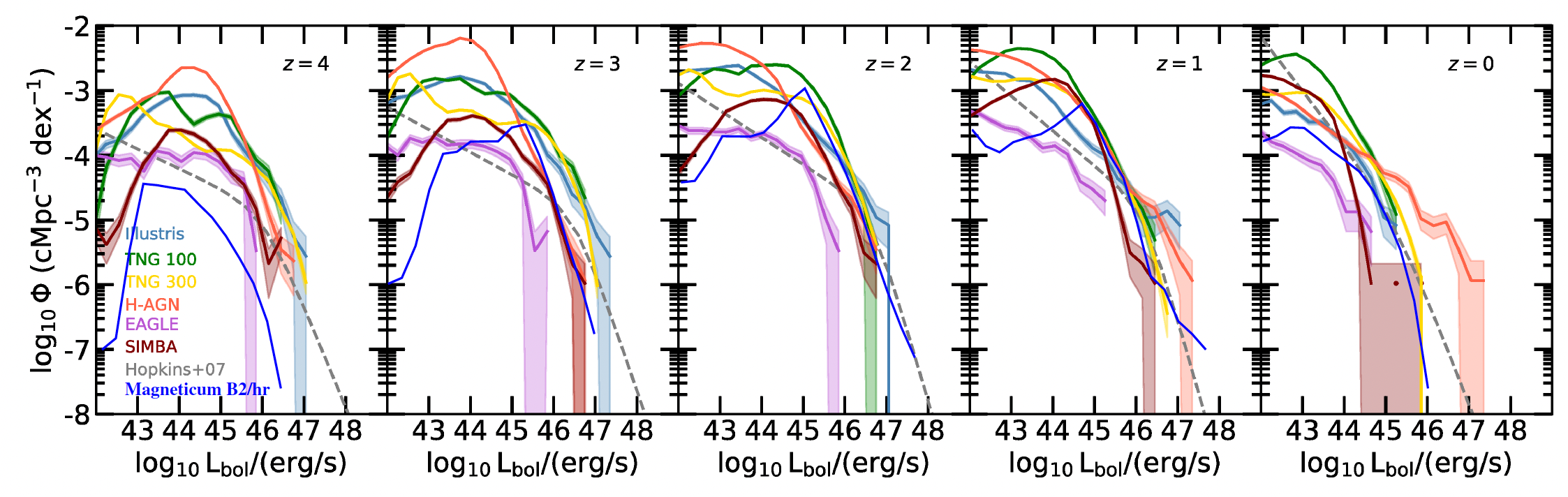
不同,现代实现通常将黑洞吸积率$\dot{M}_{\bullet}$乘以因子$(1-\epsilon_r)$予以修正。因此,$\,L_{\mathrm bol} = \epsilon_r / (1-\epsilon_r) \, \dot{M}_{\bullet} \,c^2 \,$,吸积过程中辐射出去的能量得以计及。不同的吸积率方案,加之所有亚网格过程联合作用引起的ISM/IGM性质变化,通常导致各最先进模拟之间AGN光度函数预测演化的显著差异。这在Fig. 11中进行了总结,我们可以看出模拟预测在宇宙时间尺度上如何显著偏离观测到的AGN光度函数(另见[275]
中的讨论)。
By exploting the BH accretion rate $\dot{M}_{\bullet}$, the bolometric luminosity $L_{\mathrm bol}$ can be associated to each BH in the simulation. A common assumption consists in following [273]
to distinguish between high and low BH accretion state in terms of the Eddington ratio $f_{Edd} = \dot{M}_{\bullet}/ \dot{M}_{Edd}$ (i.e. the ratio between the BH and the Eddington accretion rates) and compute:
$$
L_{\mathrm bol} =
\left\{
\begin{array}{ll}
10 \, ( \epsilon_r \; c)^2 \, \dot{M}_{\bullet} & f_{\mathrm Edd}>0.1 \\
(10 \, \epsilon_r\; c)^2 \, f_{\mathrm Edd}\; \dot{M}_{\bullet}\;\; & f_{\mathrm Edd}\leq0.1
\end{array} \right.
$$
(see [274]
,[275]
).
In contrast to the original model [242]
,[241]
, modern implementations often correct the accretion rate $\dot{M}_{\bullet}$ of the BH by a factor $(1-\epsilon_r)$. As a consequence, $\,L_{\mathrm bol} = \epsilon_r / (1-\epsilon_r) \, \dot{M}_{\bullet} \,c^2 \,$, and the energy radiated away during the accretion process is taken into account.
Different prescriptions for the accretion rate, in combination with the change of the ISM/IGM properties produced by the combined action of all the sub-grid processes, typically leads to significant variations in the predicted evolution of the AGN luminosity function among the various state-of-the-art simulations. This is summarized in Fig. 11, where we can appreciate how predictions from simulations can strongly deviate from the observed AGN luminosity function across cosmic time (see also discussion in [275]
).
评论